Key Takeaways:
- The dividend discount model is a method of stock valuation, and understanding DDM meaning is crucial for investors. It is based on the principle of the time value of money. The DDM model helps to determine whether the current market price reflects the fair value.
- The main idea is to make an investment decision based on the cash flows generated by the stock. To do this, the future dividends are summed and discounted to their present value.
- This method is best suited to stocks that pay stable dividends, such as Dividend Aristocrats. It is not possible to accurately assess the intrinsic value of a company whose distributions are difficult to predict.
In this article, we will explain ‘what is DDM’ in detail, provide the DDM formula, and give an example of its application to a real company.
Table of Contents
Understanding the Dividend Discount Model: Basic Principles
The discount model is a mathematical model for stock price valuation based on the cash flows generated by the security in question. The model is founded on the principle of the time value of money. According to this principle, $1 today is worth more than $1 in the future due to its investment potential.
This analytical method aims to determine the intrinsic value of a stock, independent of short-term market conditions. The dividend discount model assumes that the current stock price is equal to the present value of future dividend payments, adjusted by the discount rate.
From an economic perspective, the discount rate represents the required rate of return. Its value depends on various factors, including investment risk.
Theoretical Foundation and History of the DDM
John Burr Williams introduced the fundamentals of the DDM in his 1938 book. The model’s historical development was further advanced through academic research by Myron J. Gordon and Eli Shapiro. They published their work in 1956, refining and popularising this financial theory. Consequently, one variant of the DDM is now known as the Gordon Growth Model.
Despite the emergence of new methods, dividend discount models remain relevant. These financial analysis tools are still widely used to value dividend-paying stocks.
The Basic Dividend Discount Model Formula
The fundamental DDM formula is as such:
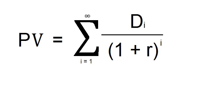
In this formula, the numerator represents the future dividends that an investor expects to receive from the stock in question. The denominator, r, is the discount rate and i indicates the time period, measured in years. PV stands for ‘present value’.
This equation is a mathematical representation of the principle of the time value of money. For practical calculations, the formula is often simplified by making the assumption that the dividend growth rate is constant.
In practice, the present value is compared with the market stock price. If the current market value is lower than the calculated present one, the stock is considered undervalued and a purchase is recommended.
Key Variables in the DDM Formula
The main limitation of dividend discount models is that they are sensitive to input variables. Even small changes to these variables can lead to significant fluctuations in the final result.
A key concern is the estimation of the required rate of return and the dividend growth rate models. When using the Gordon Growth Model, for example, the discount rate is determined as the difference between:
- The cost of equity, which can be estimated using the Capital Asset Pricing Model (CAPM).
- The dividend growth rate. For some companies, this rate is calculated by multiplying ROE by the retention ratio. For others, it is based on the assumption of steady dividend increases by the same percentage each year. When dividends are fixed, the growth rate is assumed to be zero.
The most recent dividend payment is usually used to represent expected dividends in the numerator of the formula.
Types of Dividend Discount Models
The model variations employ different approaches to calculating a company’s stock price based on dividends. They differ in terms of their complexity and the scope of their application. The most complex are the variable growth models, which assume dividend growth rates will be divided into several stages. Another model is the H-model, which accounts for gradual changes in dividend rates.
Now, let’s consider some variants of the DDM:
- Gordon Growth Model;
- zero-growth model;
- multi-stage DDM.
The best way to decide which one to use is to consider the company’s dividend payment history.
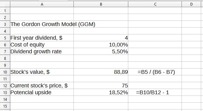
The Gordon Growth Model (GGM)
The constant growth DDM applies to mature companies that have demonstrated stable dividend growth over many years. At the same time, they must ensure that their dividend growth rate exceeds the required rate of return.
The Gordon Growth Model assumes that dividends increase at a constant rate. Because it assumes uniform and perpetual growth, the formula for DDM is in its simplest form:
PV = D₁ / (r – G).
D₁ represents the expected dividend. It is typically calculated as D₀ × (1 + G), where D₀ is the dividend for the current period, r is the required rate of return (or equity value) and G is the expected perpetuity growth rate of dividends.
Here is an example of calculation in Excel.
Zero-Growth Dividend Discount Model
The DDM is also referred to as the no-growth model. It is used to value preferred shares that guarantee fixed payouts. However, it is more commonly used to value stable companies in mature industries that pay constant dividends.
If a company does not increase its dividends in perpetuity, the calculation is performed using a simplified DDM:
PV = D / r.
Multi-Stage Dividend Discount Models
The DDM allows for multiple growth phases. A two-stage model and a three-stage model are typically distinguished. These options facilitate complex valuations. They incorporate variable growth rates of dividends at different stages of a company’s life cycle.
The three-stage model includes:
- a high-growth phase;
- a growth transition period;
- a mature phase of slow dividend growth.
The two-stage model only includes the growth phase and the stability period. The formula used in this case is as follows:
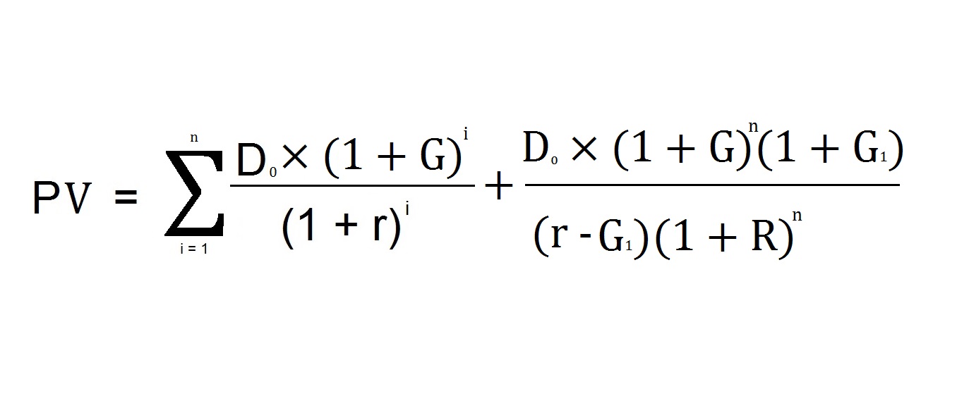
Here, G represents the dividend growth rate during the initial high-growth period of n years. G₁ represents the growth rate of shareholder rewards during the second phase. It is assumed that the second phase will significantly exceed the duration of the first.
The main drawback is the assumption that high growth in dividends will be abruptly replaced by a stable phase. The next stage in the development of the model of the growth dividend discount was therefore the H-model.
Calculating Stock Value Using the DDM Formula: Step-by-Step Guide
Let’s provide a stock valuation example using the GGM in a step-by-step process.
Step 1. Determine the constant growth rate (G). For the purposes of this example, let’s assume it is 2%.
Step 2. Find the company’s cost of equity capital. Suppose it is 5%.
Step 3. Calculate the expected dividend, D₁. Assuming that the company paid $4 this year, D₁ would be $4.08 ($4 × (1 + 0.02)).
Step 4. Calculate the expected stock price. This will be $136 ($4.08 / (0.05 – 0.02)).
Step 5. Compare the result obtained with the current fair price in order to make an investment decision.
The formula implementation for multi-stage dividend discount models is much more complex. The calculation process can only be performed through Excel modeling.
The practical application of the stable growth-based discounting model is only feasible for very mature companies.
Interpreting DDM Results for Investment Decisions
The dividend discount model DDM is easy to use in an investment strategy for decision making regarding buying:
- If the calculated fair value is higher than the market price, these are buy signals, and the securities are considered undervalued stocks.
- If the current fair value is below the market price, these are sell signals. However, it is important to remember that overvalued stocks can remain so for a considerable amount of time.
Investors appreciate the idea of discounting future cash flows because it allows for simple valuation comparisons across companies operating in different industries.
The discounted dividend model requires many assumptions and approximations to determine intrinsic value. For this reason, it is often recommended that it is used alongside other valuation methods.
Understanding DDM Meaning: Advantages and Limitations of the Dividend Discount Model
DDM benefits:
- has a solid theoretical foundation;
- suitable for investors focused on real cash flows;
- provides reasonably accurate results for companies that pay stable dividends.
Model limitations:
- Sensitivity to inputs. For example, reducing the parameter G from 2% to 1.5% in our case causes the calculated fair value to drop from $136 to $116 — a change of more than 10%.
- Irrelevance to non-dividend stocks. An even greater problem arises if the company’s cost of equity (r) is lower than the dividend growth rate. This can happen during an economic crisis, when payments are made through borrowing or using profits from previous years.
- Low valuation accuracy due to numerous assumptions. One practical challenge is establishing the growth rate of shareholder rewards. Even dividend kings do not maintain it at the same level over several decades.
- Ignoring other factors affecting stock value, such as market share expansion. Therefore, it is not advisable to use this method to evaluate growth stocks.
When to Use (and When Not to Use) the DDM
Company maturity is one of the key criteria for a valuation model selection. The appropriate applications of this method include:
- mature companies, blue chips;
- REITs, which are required to distribute a large portion of their net income;
- banks and other financial institutions;
- non-cyclical industries, such as producers of everyday consumer goods.
Inappropriate uses include:
- growth companies that reinvest all profits;
- newly established businesses that do not yet have a dividend history;
- companies with uncertain dividend payout dynamics, for which it is impossible to make assumptions about future dividend growth rates.
Valuation alternatives should be applied to such stocks.
DDM vs. Other Valuation Models
As well as the DDM, the following valuation methods are also popular:
- The DCF (discounted cash flow) model works with a company’s expected future cash flows. It does not take into account amounts received by shareholders.
- The FCFE model examines the relationship between a company’s free cash flow and its capital.
- The P/E ratio is a relative valuation metric that shows how many dollars need to be paid for each dollar of the company’s profit. It is poorly applicable for comparative analysis of companies from different industries.
The model comparison shows that all of the above-mentioned valuation methods are complementary approaches. When used together, they provide a more comprehensive analysis, making it easier to determine whether stocks are undervalued or overvalued.
Case Studies: Applying the DDM in Real-World Scenarios
To illustrate with a practical example involving a real company, consider Walmart. From 2019 to 2024, WMT increased its dividends by $0.04 each year, reaching $2.24 by 2024. This equates to a consistent growth rate of 2%.
The required rate of return can be estimated using the CAPM method. As the risk-free rate, we take the United States 10-Year Bond Yield, which is 4.4%. The stock’s beta and the desired risk premium are added. The investor’s required rate of return (r) is assumed to be 7%.
In this case, the estimated cost would be $45.60. The current price of WMT is $94.20. According to this dividend stock valuation method, the company is overvalued. This real-world application of the model shows that investment analysis must consider more than one factor.
The model case studies include sector-specific applications. For instance, it can easily be adapted for companies in the technology sector that pay low dividends.
When dealing with growth stocks, it is best to abandon the assumption that investors will hold the stock forever. Over time, investors will want to realize capital gains, so the sale price must also be considered. This can be illustrated using a one-period model.
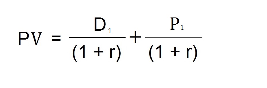
PV = (D1 / (1 + r)) + (P1 / (1 + r))
Let’s use Nvidia as an example. Suppose D₁ is $0.04 and P₁ is the terminal value at which an investor would sell the stock after one year. The consensus analyst forecast is $172.11. For growth stocks, the cost of equity is higher than for dividend kings due to higher beta and risk premium assumptions. Assuming r equals 9%, the valuation results are approximately $158 (($0.04 + $172.11)/(1 + 0.09)).
Common Mistakes and Misconceptions About the DDM
The most common modeling errors include:
- incorrect future dividend growth assumptions;
- company’s cost of equity valuation errors (required rate of return);
- misapplications of model modifications to a specific company;
- input mistakes and technical challenges with calculations involving complex formulas.
Another popular misunderstanding relates to the misinterpretation of results. This often stems from methodology issues, such as the valuation approach not accounting for important market factors. For example, the price of a company’s stock based on dividends is not applicable to growth companies.
DDM Meaning and The Future of Dividend Discount Modeling
One of the advantages of the dividend discount model DDM is its capacity to incorporate evolving approaches and technological integration. Modern adaptations and model enhancements allow for the elimination of limitations. Using AI in valuation improves calculation accuracy. Contemporary applications for automated valuation save investors from labor-intensive computations.
Conclusion: Mastering the Dividend Discount Model
Key takeaways and final thoughts:
– The practical implementation of the discount dividend model is challenging due to the variability of the factors involved.
– For investors seeking to understand DDM meaning, it represents a valuation method that estimates a stock’s intrinsic value based on the present value of its future dividend payments.
– Valuation mastery with this method depends on the investor’s understanding of the CAMP model, determines the required rate of return, and makes dividend growth rate assumptions.
– DDM is an important component of the investment toolkit used for company valuation.
However, it is not a universal method. To use the model properly, the model integration into a comprehensive valuation framework is required. The expected value based on DDM should not be the sole criterion for making a purchase decision.
FAQ
H3: What is the difference between CAPM and DDM?
The CAPM model relates risk to a business’s expected return. The DDM meaning is an estimate of the present value of the future real cash flows that a stock will generate for its owner. While these are not interchangeable, they are complementary methodologies.
What is the 3 step dividend discount model?
This model considers different growth phases of dividends when valuing companies. These include a high growth period, a transition phase, and a period of slowly growing or stable dividends.
What is the dividend discount model ratio?
The variable r is used in the fundamental formula and its modifications. This represents the rate of return that an investor expects to receive in exchange for investing in stocks.
What is the DVM calculation?
This refers to establishing the current fair price of a stock based on the passive income it is expected to generate.
Article Sources
- Gordon, M. J., & Shapiro, E. (1956). “Capital Equipment Analysis: The Required Rate of Profit.” Management Science, 3(1), 102-110.
- Damodaran, A. (2012). “Investment Valuation: Tools and Techniques for Determining the Value of Any Asset.” John Wiley & Sons, 3rd Edition.
- Foerster, S. R., & Sapp, S. G. (2005). “The Dividend Discount Model in the Long-Run: A Clinical Study.” Journal of Applied Finance, 15(2), 55-75.
- Fuller, R. J., & Hsia, C. C. (1984). “A Simplified Common Stock Valuation Model.” Financial Analysts Journal, 40(5), 49-56.